
WYCKOFF · C / D
Wyckoff distribution: UTAD and SOW
An upper wick and a red candle do not describe a complete range. Separate the observation at resistance, the return inside and the later move toward the lower boundary. The educational schematic gives an order for comparison; the live scanner supplies timestamps and inspectable labels.
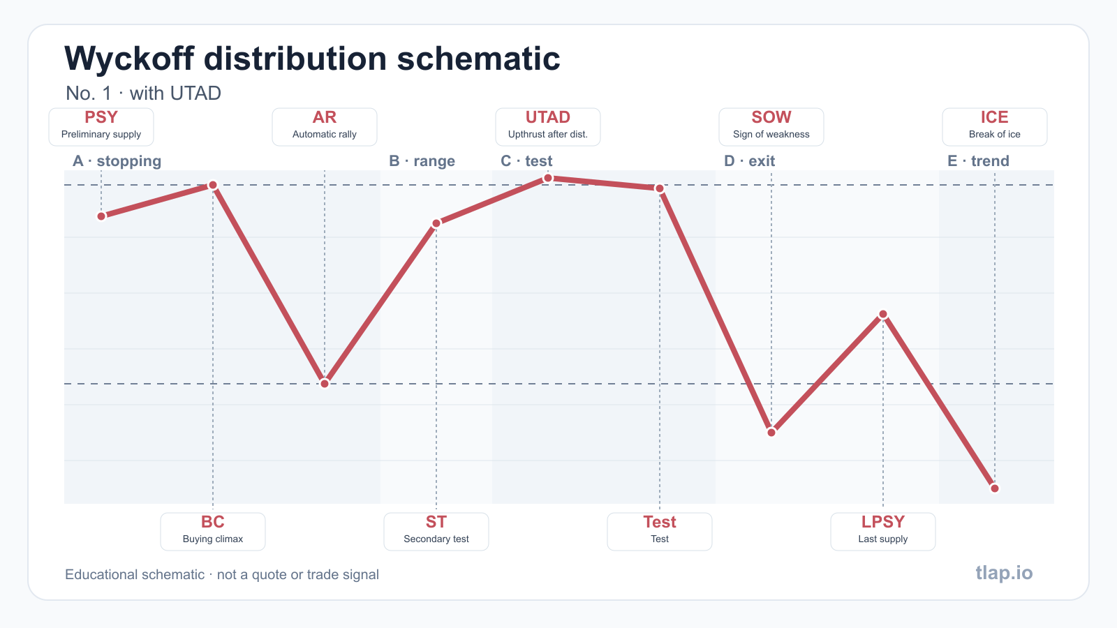
UTAD and SOW in the schematic
UTAD describes a late false excursion above the range; SOW denotes a sign of weakness. They concern different observations: a test of the upper edge and a subsequent move should not be merged into one candle simply to match a drawing.
Start with both boundaries of a specific active structure in the scanner. Compare the resistance-test time with later closes. When a structure closes or is recalculated, its older events remain historical observations; they cannot be presented as the current range.
What the live summary selects
The block below shows active distribution structures in C and D. Phase C alone does not establish a UTAD: schematic No. 2 allows a different sequence without that late event. Open the scanner and read its actual labels; current phase and last-event type are separate fields.
Check the ticker together with its timeframe. Distribution on 4H does not automatically describe the same instrument on 1H or 1D. If the summary is unavailable, the number of matching ranges is unknown. Zero is shown only when a complete fresh response contains no matching rows.
Returning to a boundary
After a move toward the lower edge, record the closes, then consider any return separately. Do not carry an old structure's upper boundary into a new one or name every rally after a decline LPSY. A repeatable comparison retains time order and data provenance.
A proxy-volume label matters when interpreting an observation. It does not change the price boundary, but limits conclusions about traded volume. Compare both distribution variants in the atlas: similar final drawings do not establish identical event sequences.
Separate the drawing from the outcome
The schematic ends with downward movement, yet a real confirmed event may be cancelled or fail to reach its target. Inspect its outcome separately in history. A C/D summary locates current observations; it does not supply a probability, an execution price or a finished result.
An upthrust within the range and a late UTAD
First identify the range you are examining. Record its start and both boundaries, then locate the event on the selected timeframe. An excursion near resistance does not explain the entire preceding structure by itself. Check the phase in which it appeared, whether price returned inside, and whether the same markup remained after that test. A boundary from the four-hour chart and an event from the hourly chart cannot be combined and presented as one scanner sequence.
In the variant with a UTAD, the late test above the upper boundary belongs to phase C. The variant without a UTAD is a separate sequence, not a defective copy of the first drawing. Compare the labels that actually exist rather than adding a missing event to make the chart resemble the picture. A SOW and the transition to phase D are checked separately. Read LPSY in the context of a subsequent return; every green candle is not a last point of supply. An open candle can still change, so use closed bars and the times displayed in the panel.
Repeat the comparison on the live chart
Open an instrument from the summary and keep the same timeframe. Check its market identity, latest closed-bar time and feed status. A delay message means that available closed bars lag behind the expected schedule. An undetermined schedule describes another limitation: the scanner cannot reliably establish freshness. Until that limitation is resolved, the absence of a new event does not establish a quiet market. Neither state should be replaced by a fabricated zero or an assumption that the provider has stopped trading the instrument.
Next compare price with both boundaries of this particular range. Read the latest event, phase and status, then open history. Distinguish its initial record from later recalculations. A subsequent rule clarification can change a label or outcome without making that new version information that was available earlier. When an event is cancelled, the retained record explains the change. Its disappearance from a current summary is not a reason to erase its history or describe it as a new observation.
Finally return to the schematic and compare order rather than the scale of its illustrated movements. The educational line specifies no actual prices, phase duration or size of the next move. Distances in the drawing are neither a forecast nor a stop-placement rule. A ticker, timeframe, event time and range identifier provide a repeatable reference. Another reader can use that combination to inspect the same context instead of trying to recognise an approximate visual resemblance.
Read the origin of the adjacent statistics
Each statistical row has a source. A journal snapshot includes earlier history recorded under the rules in effect on its snapshot date. Live observations appearing after that date form a separate population. Recalculating two years of retained history under current rules answers a third question: how the algorithm labels those stored candles now. Compare the row labels and denominator n before comparing percentages. The complete historical baseline cannot be presented as events observed live during the few days since the journal was created.
With few completed cases the scanner reports insufficient data. If it falls back to an asset-class and timeframe aggregate, that source is distinguished from the individual instrument sample. Target attainment, invalidation and no result refer to the defined window of the next thirty closed bars. These describe outcomes of labelled cases; they do not provide a ready probability of a profitable trade. Proxy-volume feeds retain another limitation: their values cannot establish measured exchange turnover, and missing observations must not be reconstructed from assumptions.
FAQ
Does distribution require a UTAD?
No. The atlas includes a variant without UTAD. Phase C alone does not identify a specific variant.
Why is SOW not a finished outcome?
It labels an observation. The outcome is measured later and stored separately from the current phase.
Why can an instrument disappear from this summary?
Inspect the new snapshot and history: its range can change phase, close, become stale or be recalculated.