Risk of Ruin, or How Not to Blow Up While Trading Monkey Bots

You've probably already heard a lot about martingale, grids, and other spectacular ways to blow up your deposit. And indeed, these are systems that, even purely theoretically, will not allow you to win consistently. However, there are many traders, including experienced ones, who use grids on their accounts. Do you think they don't know the theory? Of course they do, there's just a little secret. And that's what we'll talk about today.

The fact is that most retail traders have rather modest accounts, and very often they choose quite aggressive methods of capital management. Grids and martingales do indeed quite often lead to the loss of the entire deposit, but experienced traders always advise periodically withdrawing part of the profits. In this way, we get more or less stable earnings from trading systems that, it would seem, are doomed even in pure theory. Today we will find out why this happens from a mathematical point of view and learn how to extract the maximum benefit from this "miracle."

This very "miraculous way" of making money on losing strategies can be used quite well with a scientific approach; you just need to familiarize yourself with the concept of probability of ruin.

Knowing the probability of ruin for a specific trading system with the selected money management method, you can more or less accurately say whether a trader will blow up or not. Many traders, especially beginners, are always in a hurry, as if the markets will soon close and they will not have time to earn their millions for a comfortable life. As a result, the probability of ruin goes through the roof and, accordingly, another account is lost.

Probability of ruin, or probability of ruin, abbreviated POR, is the statistical probability that the trading system will cause an account to go bust before reaching the dollar level considered successful. Ruin is determined by the account level when traders stop trading. POR illustrates to traders the statistical possibility of their trading systems shifting toward success or ruin.

Some authors believe that interest in the probability of ruin is misplaced because it does not provide traders with insight into how to make a profit. In this sense they are right. In addition, the probability of ruin tends to be small in truly profitable trading systems. However, if all other aspects are equal in importance, then when choosing between two trading systems, you will most likely choose the one with the lowest probability of ruin.

Most often, in long-term profitable systems risk of ruin is quite low. Rarely does it reach the 5% mark. As a rule, these are trading systems that have sufficient capital and bring profit to the trader. It is not uncommon for beginners to have a POR in the 70-100% range, which means that the account will definitely be blown up, even if they tell you that they have finally found a holy grail trading system. POR is not a constant value, and for normal traders it stays in the 0 to 5% range most of the time. But if you see that this indicator has increased, most likely you have started taking too much risk. In that case, it is enough to simply reduce the risk in each trade, and then the probability of ruin will return to an acceptable level.

Below you can see the risks of ruin when using hard stops. The calculation takes into account the probability of winning in each transaction and the ratio of profit to loss.

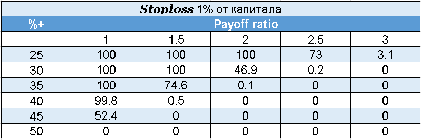
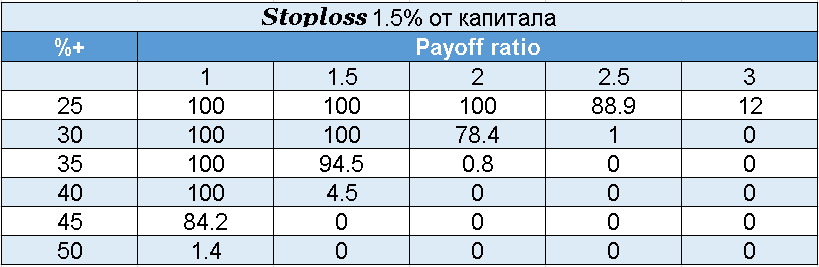
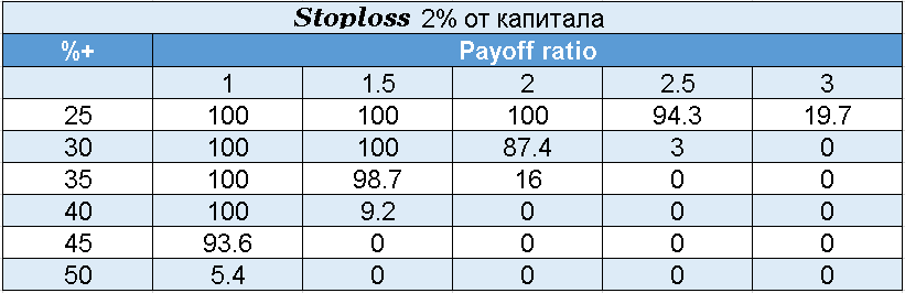It is important to take into account that the stops for calculation were taken to be fixed, and the probability of obtaining a winning trade was constant over time, although in reality this, of course, is not the case.

Calculation formula

I will give the simplest formula for calculating the probability of ruin:

Where q is the probability of “failure”, the loss from which in each individual trial is equal to -1;

p is the probability of “success”, the profit from which in each individual trial is equal to +1.

Q(z = 0) is the probability of ruin occurring when the initial capital (z) becomes equal to 0. Then P(w) = 1 - Q(z = 0) is the probability of achieving the goal (increasing the initial capital (z) to the value w).

As you can see, it does not take into account the magnitude of winnings and losses. That is, such a formula can only be applied to systems in which winnings are always equal to losses.

Let's look at an example. We have 100 bucks, and our system gives 45% profitable trades. Then q = 0.55 and p = 0.45. We want to know with what probability we can achieve 100% profit, or $100 profit, with this system.

Q = ((0.55/0.45)^200 – (0.55/0.45)^100)/((0.55/0.45)^200-1) = 99.(9)%, that is, almost 100%.

And the probability of success is P(w = 100) = 1 - Q(z = 0) = 0. A zero probability of success means a definite loss of the account even before 100% of the profit is achieved.

However, it turns out that if your goal is to win just one dollar, then the probability of success in this is:

P(w = 100) = 1 - Q(z = 0) = 0.818 or almost 82%.

Accordingly, no matter how bad the system is, the larger the trader’s initial capital, the greater the chances of winning a small amount before he goes broke. Even with an unfavorable probability of success on any given attempt, the odds of a trader winning a small amount before going broke can be significant. And the higher the initial capital, the higher they are.

In this regard, it is of interest to make a more detailed assessment of the change in the probability of ruin depending on the gradual increase in the rate in unfavorable conditions (q>p). Omitting mathematical calculations, we note that while the initial capital remains unchanged, a gradual increase in the rate leads to a decrease in the likelihood of ruin for the doomed trader. Accordingly, the probability of ruin for someone whose success is guaranteed according to mathematical expectation increases.

This can also be formulated as follows: in a repeated game with a constant bet, the probability of ruin will be minimal when choosing a bet that was compatible with the amount of the desired win.

For example, we have z = 90 dollars, but we want to get w = 100 with the same probabilities q and p.

Q = ((0.55/0.45)^100 – (0.55/0.45)^90)/((0.55/0.45)^100-1) = 0.866 or 87% probability of losing the account.

But if we increase the bet to the maximum possible value (in this example we need 10 dollars and z = 9, w = 10), then such an unfavorable forecast can change significantly.

Q = ((0.55/0.45)^10 – (0.55/0.45)^9)/((0.55/0.45)^10-1)= 0.21

And although the mathematical expectation of winning remains the same, the probability of ruin will be only 0.21, and the probability of winning will increase to 0.79.

As we can see, despite the unfavorable ratios of p and q, the doomed trader has significant chances of emerging victorious in one of the attempts. Of course, this victory can only be preserved if the trader has the opportunity to leave trading with the winnings.

An even simpler formula is obtained for tests with an ideal coin, when p=q=50%:

Q(-z) = 1 - (z/w),

where (w - z)>0 – “net” gain.

Then the probability of this outcome:

P(z) = 1 - Q(-z) = z/w.

If we examine the dependence of the function Q(z/w) on the ratio of the variables z and w and plot a graph, we find the following:

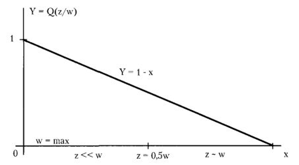For a given constant value of z (z = const), the probability of ruin decreases as the value of w changes towards closer to z. And the probability of ruin reaches its minimum values ​​when the values ​​of w and z become comparable (z - w).

When p = q, the probability of ruin Q becomes minimal, and the probability of winning P becomes maximal under two conditions. This is the minimum winning goal and the maximum bet.

For example, with a bet of 0.1 z we get w = z + 0.1z and Q(-z) = 0.09, and the probability of winning is 91%.

Let's look at another example. Let the player have an initial capital of $3000. The stake (stoploss = takeprofit) for each game is $300. Then we have the conditions: z = 3000 and w = 3300. But since the value of $300 serves as one "notional unit," on the calculation scale used above this means that z = 10, and w = z + 0.1z = 11. And we arrive at the conditions and solutions of the previous example, where: Q(-z) = 0.09 and P(w) = 0.91.

Let's now look at an example of putting a monkey bot on an account. I think this is the example that interests everyone most. We have $1000, and we will put the expert advisor on a $100 account. Our primary task is to withdraw the first 100% of profit, after which we will be back to breakeven even if the account is blown up later. In this case, z = 100% (our 1,000), and w = 110% - we need to make a profit of 10% of the initial deposit. Then we can write it like this: z = 10, w = 11. Let's assume that we do not know the future and that we are just as likely to lose our $100 stake as to earn 100% on it. That is, on average, in half the cases we will blow up our accounts. Then:

Q(-z) = 1 - (z/w) = 1 – 10/11 = 0.09, or 9% chance of running out of money. At the same time, the chance of ending up with $1,000 in hand and a profit of $100 is 91%.

If in at least 60% of cases we do not lose our hundred, which will mean that we have received the entire safety deposit back and we have a bot working with a hundred that we no longer mind losing, then the probability will be much higher:

Q = ((0.4/0.6)^11 – (0.4/0.6)^10)/((0.4/0.6)^11-1)= (0.01156 - 0.01734)/(0.01156 - 1) = 0.00585, or 0.6% risk of ruin. Then the probability of making a profit will be 99.4%.

To better understand this approach, let's now take the initial capital to be $400 and p=q=0.5. Then z = 3 and w = 4:

Q(-z) = 1 - (z/w) = 1 – (3/4) = ¼ = 0.25, or a 25% probability of losing all funds before we manage to withdraw the hundred. After that, with a 75% probability, we will again have our $400 in hand, while $100 will remain working on the monkey-bot account. What's next? Then you can simply withdraw profits from this account and not worry about the account blowing up again. Indeed, in this case, you will have recovered your own money and can simply repeat the cycle with an initial capital of $400.

As we see, with an unfavorable ratio p<q it is possible, by manipulating the values ​​of w, z and the size of the bet, to achieve impressively good proportions Q(z) and P(w).

In this regard, the question arises about what is the mathematical expectation of the result, i.e. the average payoff during a long repetition of the game, under conditions of an unfavorable ratio p<q and favorable ratio Q(-z)<P(w).

As follows from the conditions, the final result of the game (“victory” w or “defeat” z = 0) is a random variable that takes one of two values: (w-z) or (-z).

Then the mathematical expectation of gain M for any, including equal, ratio q and p:

M = P(w) * (w - z) - Q(z = 0) * (-z) = w x P(w) - z.

And for q = p:

M = w * (1-Q(z = 0))-z.

If we substitute the values ​​of Q(z = 0) into these formulas, we get:

M (for q>p)<0

And

M(q = p) = w X {1 - Q(z = 0)} - z = w X (z/w) - z = 0.

Knowing these calculations allows you to choose the “lesser evil”. Thus, the following important rule must be taken into account: if the trader is in unfavorable conditions p<q and sets the task to finish either after he wins the amount w, or loses the maximum allowable amount z, then no relations Q(-z)<P(w) will not change the negative mathematical expectation of the result.

So, no manipulations with these variables allow us to count on a positive value of the mathematical expectation. Worse, even zero is unattainable.

Thus, the procedure for applying a rational method of managing a case can be as follows: for a given ratio of p and q, a specific version of the ratio of the values ​​of w and z is calculated, at which the maximum mathematical expectation (“the least evil”) is achieved. For given p and q, it is worth choosing such ratios of the variables w and z that provide the best mathematical expectation. However, let us recall that we are talking about the mathematical expectation of the result under the condition of an infinite number of tests.

In this regard, it is useful to consider estimates of the average duration of the game at which, according to probability theory, predetermined goals can be achieved. And this duration parameter should also be taken into account in the management process.

We present without derivation the basic formulas for estimating the average duration of a game for different ratios p and q.

For the case when q is not equal to p (p>q or p<q) and with the size of the initial capital z, and the goal w (in each game the bet is one notional unit), solving the equation leads to the formula:

Let us return to the above example, in which there is a situation of a “disadvantageous” game at q = 0.55 and p = 0.45 (z = 90, w = 100 “arbitrary units”). We have already seen that if during each test the bet is equal to one "notional unit", then the probability of ruin is Q(z) = 0.866. Then the probability of winning is P(z) = 0.134.

Using the formula for calculating the average duration of a game, we find that its mathematical expectation will be:

D(z/w) = 767 trials.

However, if we increase the bet to the maximum, making it equal to 10 "notional units", then we get:

Q(z) = 0.210, a P(z) = 0.790.

And the mathematical expectation of the game duration:

D(z/w) = 11 trials.

The corresponding rule can be formulated as follows: the smaller the mathematical expectation of the duration of the game, the greater the probability of winning with an “unfavorable” ratio q>p becomes more and more favorable.

The shorter the expected duration of a “disadvantageous” game, the better. This calculation corresponds to the law of large numbers: the greater the number of trials, the closer the results will be to the mathematical expectation of the probability of “success”.

For q = p another formula is valid, which has the form:

D(z/w) = z x (w- z).

Let us immediately note that the average duration of a game turns out to be much longer than “common sense” tells us.

So, if q = p, then with the initial capital z = 90 notional units and the player’s desire to bring this amount to w = 100:

D(z = 90 / w = 100) = 90 x 10 = 900.

Note that with a bet of 10 “standard units” the probability of “success” is very high:

P(z = 90 / w = 100) = 90 / 100 = 0.9.

However, it will take a lot of time to get one or another result (ruin or a “net” win of 10 units).

Even if the player sets such a modest goal as the “final win” of just one "notional unit" (w = z + 1), then the duration of the game with capital z = 90:

D(z = 90 / w = 91) = 90 x 1 = 90.

At the same time, the probability of “success” is extremely favorable:

P(z = 90 / w = 91) = 90 / 91 = 0.99.

Let us pay attention to the fact that, despite the high probability of winning, there is a long struggle ahead (on average 90 trials). And this is in order to get a gain equal to just one unit of capital.

However, the comforting thing is that one "notional unit" of capital may amount to a significant sum of "real" money. True, in that case you would have to deploy initial capital 90 times greater than the winnings.

As we see, it is impossible to predetermine the most “profitable” path: a lot depends on various circumstances.

Let's go back to the example above, but let's take $300 as one “notional unit”.

Then the random variable D(w/z) taking into account the new “unit” is calculated using the formula:

D(w/z) = (z / 300) x (w - z) / 300.

Let's consider the expected duration of the game depending on what goals the trader sets.

If you want to win $300, i.e. 10% of the initial capital, we get the following estimates:

- probability of winning:

P(z = 3000 / w = 3300) = z / w = 3000 / 3300 = 10/11 = 0.91;

- game duration:

D(w = 3300 / z = 3000) = (z / 300) x (w - z) / 300 = 10.

Let's compare this result with other conditions.

If the goal is to increase your capital by 20% with the same bet of $300 in each game:

- probability of winning:

P(z = 3000 / w = 3600) = 10/12 = 0.83;

- game duration:

D(w = 3600 / z = 3000) = 20.

For double “enrichment” under the same conditions:

- probability of winning:

P(z = 3000 / w = 6000) = z / w = 0.5;

- game duration:

D(w = 6000 / z = 3000) = 200.

Thus, the above calculations again confirm the estimates obtained earlier: the more ambitious the goals, the less likely their achievement becomes.

At the same time, the duration of the game increases faster than intuitively expected. In the example above, you can see that increasing the target size from 20 to 100% (five times) increases the average game length from 20 to 200 trials (ten times).

Increasing the profit goal, all other things being equal, leads to a decrease in the probability of winning and a disproportionately large increase in the duration of the game.

And finally, let's calculate the expected duration for our example with monkey bots installed on accounts. So, we have an initial capital of $400 and each time we place $100 into the account. The probability of losing all the money is quite high: Q(-z) = 1 - (z/w) = 1 – (3/4) = ¼ = 0.25. D = 3/(4-3) = 3, that is, on average, a similar outcome will be achieved in 3 bets.

The probability of ruin is not so necessary for traders who trade using classic money management systems. If a trader calculates the risk of ruin, it is possible to determine whether he is taking too much risk at the moment, and also whether he has too little capital to start trading using the new system.

The greatest benefit from this knowledge can be gained by traders who use dangerous systems and expert advisors. It lies in the fact that you can calculate the risk of ruin across a series of runs of dangerous expert advisors, the expected profit from that, the number of attempts in the series, and the probability of going broke. Of course, I don’t encourage you to rush to install dangerous expert advisors on your accounts, but if you are already doing this, then I suggest taking a more scientific approach than playing in a casino.

Without delving into the above formulas, I would like to once again say in a few simple words about the benefits of calculating the probability of ruin.

If you don't mind various mathematical calculations, you can quite simply calculate a money management strategy for dangerous expert advisors: the initial capital, the average number of attempts, and the mathematical expectation of your strategy. If formulas bore you, just use the calculations that were given in this article as examples. All this data and these calculations lead to one very simple rule: to launch a dangerous bot safely, you need initial capital 10 times greater than the deposit required for the advisor. This will let us recover our investment almost for sure and possibly start making a profit.

Best regards, Dmitry aka Silentspec TradeLikeaPro.ru