How to Calculate Optimal F: Step-by-Step Risk Percentage Guide

Greetings fellow forex traders !

There is a belief that Optimal F is the single best money management method. The concept of “optimal f” is probably known to every currency speculator who has ever had any serious interest in money management and capital management. The main popularizer of this idea, the American author Ralph Vince, is well acquainted with Larry Williams, the legendary futures trader. Vince himself is not a practicing trader, and many people reproach him for that. Today we will delve into this topic in detail, analyze the pros and cons of the optimal fraction method, the calculation, as well as consider modifications of the approach.

Ralph noticed an error in Kelly’s criterion, namely that the formula was originally intended to determine the direction of electron particle flow and was later used for blackjack. The trouble is that blackjack is not at all the same as trading stocks or currencies. In blackjack, your potential loss on each bet is limited to the chips you wager, while your potential winnings remain always the same in terms of chips wagered.

When we are in the market, the size of our wins and losses is constantly changing. Sometimes we get big wins, sometimes tiny ones. Our losses are subject to the same law – their size is random. Ralph came up with a formula similar to Kelly’s formula, which he called “optimal F”, but unlike Kelly’s formula it can be adapted to trading in the markets.

Optimal F (derived from the word “fraction”) is the fraction of the deposit at which we will have maximum profit. Naturally, the optimal f is not a constant value, and as trades are made, the value will change. That is, it is necessary to recalculate it.

If we graphically represent the change of the final deposit (TWR) from the size of the percentage of funds utilization (F), the dependence will be described by a curve:

As you can see, if we invest too small a part of the deposit, we will also have a small profit. If we increase the risks, the value of the final deposit will also increase up to a certain point. If the risks increase further, the final deposit will start to fall. This very moment, when the deposit growth is maximum, exactly corresponds to the optimal f. Thus, it is quite logical to assume that the optimal solution for a trader is to use such a percentage of the deposit for each trade as will be at the upper extremum of this curve.

Well then, let’s generate a random trading system for our research.

The main statistical indicators of the system are as follows:

When creating the TS, I used the generator of random numbers according to the normal distribution:

The mathematical expectation of our trading system is a little more than 1, and the standard deviation is about 4, which is quite suitable for our purposes.

Now we will introduce a money management system – in each trade we will risk a certain percentage of our capital (in this case 3%):

All we have to do is find the percentage of risk at which our final balance will be maximized. For this purpose, we can, as usual, use the solution search function built into Excel, which found the optimal value of 20%:

For the calculation we usually use not the value of the final capital, but TWR. This is an indicator that characterizes the relative final capital, or, simply put, how many times we have increased our initial deposit. And in this example, the maximum TWR was 8159238.337 at 20% risk. In other words, the optimal f specifically for this system is 0.2.

As you have seen on the chart at the beginning, the optimal f is, in fact, an extremum, above and below which there are suboptimal TWR values:

You can see from the chart that the optimal F for our system is 0.2 or 20% risk per trade. In this case, if we lay down a risk of 21%, it will give the same final result as if we risked 18%. At the same time, if we add literally one more percent and risk 22%, the account will be drained.

Let’s take a closer look at the calculation of optimal f. To calculate the optimal f, we must first calculate the profit for a certain period – HPR.

HPR=1+f*(-deal/most loss), where:

f – risk in each transaction;

deal – profit or loss in a particular deal (in case of a loss, the expression in brackets will be negative, as well as the total value);

the largest loss – the largest loss per deal (negative number).

Next, TWR is calculated as the product of all HPRs, i.e.:

TWR = HPR1*HPR2*….*HPRn, where n is the last trade in your sample.

Well, and finally, we calculate the geometric mean HPR (G), which is calculated as the root in degree n of TWR: G=TWR^(1/n), where n is the total number of deals.

We know all the parameters for calculation, except for the value of f. Your task is to step-by-step search f from 0.01 to 1 in such a way as to find the maximum G. The f at which G is maximized will be the optimal f.

Many professionals use a fixed percentage when trading, but that percentage has never been even close to as high as the optimal f. The fact is that Ralph Vince is undoubtedly a professional in his field and an excellent theorist. But one detail is highly stressful. The fact is that no matter how much we try to predict the size of the maximum losing trade, there is always a considerable probability that this value may be exceeded in the future. We can more or less well predict average values like mathematical expectation or average profitable trade if we have enough statistics. But the maximum losing trade, maximum profitable trade, and maximum drawdown are all rather poorly predictable values. That’s why the optimal f is not so useful, because if we are a little bit wrong in this maximum losing trade, we will be wrong in the optimal f. And if we are wrong in the optimal f by just a percent or two, we get a margin call.

Still, we cannot say that this formula is completely useless. Moreover, in some special cases, for example, for binary options or for systems with rigid stops and profits (although, in my opinion, such systems are suboptimal in themselves), it is accurate. Therefore, if you know exactly your maximum loss, this method of money management will work for you.

Let’s check my point of view – let’s generate another 1000 trades with the same characteristics: an average value of 1 and a standard deviation of 5. We will use the same optimal f equal to 20%.

Let’s add 1000 trades:

And let’s look at trading at the same 20% risk:

As you can see, this level of risk is no longer optimal. It has simply changed.

Let’s assume that the optimal fraction for the previous 100 trades was 15%, in the next 100 trades this fraction may be 9%. If the optimal fraction for the previous 100 trades was 15% and you decide to make the next 100 trades with the same fraction, you may well make a mistake and easily exceed the limits of the amount on your trading account.

Practical application of the optimal fraction strategy optimizes past trades. So the next trade is immediately put into the sequence and the optimal fraction is re-optimized. And will be optimized at the conclusion of each trade. That is, in real trading you will have to recalculate the optimal fraction after each trade.

In addition, trading is completely unpredictable, despite all the indicators that can be calculated on the basis of available statistics. With logic, all we can do is draw certain conclusions about reasonable expectations and probabilities. No mathematical expression can guarantee us that out of N number of trades 50% will be profitable and the other 50% will bring losses. Trading strategies are formed based on logic and to a large extent market statistics. Market behavior changes. What seemed favorable yesterday may become dangerous today.

In order to avoid draining the deposit at a small deviation, the diluted optimal f method (diluted optimal f) was proposed. In essence, diluted optimal f is a percentage of the optimal f. This technique is used, firstly, so that as a result of optimization on historical data the optimal capital value was not overestimated and, secondly, so that the trader could regulate his risk (the amount of capital used in trading) when using the optimal f.

The calculation formula is very simple:

Diluted optimal f = Optimal f * X, where X is your chosen percentage of optimal f.

You can, for example, set X = 0.5 and be sure that half of the optimal f calculated on the history will hardly ever exceed the real optimal f in the future.

The disadvantages are the same as with the optimal f, but the probability of risk overestimation, which can lead to account collapse, is much lower in this case.

Secure fraction (Secure f) is the portion of capital involved in each trade while limiting drawdown and maximizing profit. The Secure fraction has some advantages over the optimal fraction because it relies on some other factors rather than the maximum loss. The strategy is similar to the optimal f technique with the only difference being that with optimal f your strategy is optimized for profit based on the maximum drawdown over the estimated period of historical data, while with safe f you limit the drawdown yourself.

The calculation is pretty simple too. Instead of the maximum losing trade, we simply use the maximum drawdown in the currency. Working with the safe fraction method is less risky than using the optimal fraction, but capital growth will be much slower, especially on small deposits.

Today we have familiarized ourselves with such methods of money management as optimal and safe fraction. From the point of view of logic and math, both of these methods of calculating risk look very attractive. However, as we have seen today, these methods have their disadvantages as well. A great number of traders in the forex market believe that they should risk as much as possible and direct their efforts to the maximum deposit growth. In other words, there is a very large number of so-called deposit maximizers. And for them such methods of capital management as optimal fraction and Kelly criterion may seem to be an excellent solution.

For those traders who also do not mind high risks, but do not like to lose deposits too often, I can recommend using a lighter safe fraction or a diluted optimal fraction, which will eliminate the possibility of applying too much risk.

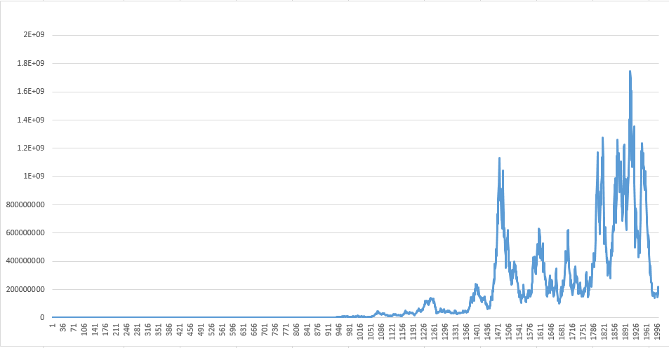Kak vidite, optimalnym etot uroven riska uzhe ne nazovesh. On prosto na prosto izmenilsya.

Dopustim, optimalnaya fraktsiya dlya predydushchikh 100 sdelok sostavlyala 15%, v posleduyushchikh 100 sdelkakh eta dolya mozhet okazatsya ravnoy 9%. Esli dlya predydushchikh 100 sdelok optimalnoy byla dolya 15% i vy reshili provesti 100 sleduyushchikh sdelok s toy zhe fraktsiey, to vy vpolne mozhete oshibitsya i legko vyyti za predely summy na vashem torgovom schete.

Prakticheskoe primenenie strategii optimalnoy fraktsii optimiziruet proshlye sdelki. Poetomu ocherednaya sdelka srazu popadaet v posledovatelnost, i optimalnaya dolya povtorno optimiziruetsya. I budet optimizirovatsya pri zaklyuchenii kazhdoy sdelki. To est v realnoy torgovle vy posle kazhdoy sdelki dolzhny budete zanovo rasschityvat optimalnuyu fraktsiyu.

Krome togo, torgovlya sovershenno nepredskazuema, nesmotrya na vse pokazateli, ko­torye mozhno vychislit na osnove imeyushcheysya statistiki. S pomoshchyu logiki my mozhem vsego lish sdelat opredelennye vyvody otnositelno razumnykh ozhidaniy i veroyatnos­tey. Nikakoe matematicheskoe vyrazhenie ne mozhet nam garantiro­vat, chto iz N kolichestva sdelok 50% budut pribylnymi, a ostalnye 50% prinesut ubytki. Torgovye strategii for­miruyutsya na osnove logiki i v znachitelnoy stepeni rynochnoy stati­stiki. Povedenie rynka menyaetsya. To, chto vchera predstavlyalos blago­priyatnym, segodnya mozhet stat opasnym.

Naydet­sya eshche sotnya drugikh i dostatochno logichnykh prichin, pochemu metod op­timalnoy fraktsii bezuprechen s matematicheskoy tochki zreniya, no okazyvaetsya dovolno opasnym v prakticheskom primenenii. Odnako nekotorye momenty, kotorye ya analiziroval vyshe, pokazyva­yut, chto net smysla prodolzhat obsuzhdenie etoy temy dalee. Risk sam po sebe yavlyaetsya dostatochno veskim argumentom protiv togo, chtoby ispolzovat metod optimalnoy fraktsii. Esli vy schitaete, chto su­meete spravitsya s riskom, to ubedites v tom, chto khorosho ponimaete etot metod, prezhde chem nachnete primenyat ego v svoey torgovoy praktike.

Itak, osnovnaya problema optimalnoy fraktsii, kak vy uzhe ponyali, sostoit v ee privyazke k maksimalnoy ubytochnoy sdelke.  V sluchae ispolzovaniya zhestkikh stop lossov eto ne strashno, no, kogda vykhody iz sdelok v ubytochnoy zone v osnovnom proiskhodyat po signalam s rynka, optimalnaya f stanovitsya ne optimalnoy i zavyshennoy, chto grozit slivom depozita ili zhe sereznymi poteryami.

Predpolozhim, v techenie torgovogo dnya proizoshlo sobytie, vyzvavshee na rynke shok, i do etogo shoka volatilnost byla dostatochno nizkoy. Samo soboy, v takikh usloviyakh vasha optimalnaya f budet ochen vysoka i velika veroyatnost togo, chto vy v etot samyy neudachnyy den voydete v rynok s riskom protsentov tridtsat, kotoryy obernetsya v itoge vo vse 50% ubytka.

Imenno po perechislennym vyshe prichinam i ispolzuyut razlichnye modifikatsii metoda optimalnogo f, s kotorymi my seychas i poznakomimsya.

Dlya togo, chtoby izbezhat sliva depozita pri nebolshom otklonenii, byl predlozhen metod razbavleniya optimalnoy fraktsii (diluted optimal f). Po suti - razbavlennaya optimalnaya f yavlyaetsya protsentnoy chastyu ot optimalnoy f. Dannaya tekhnika ispolzuetsya, vo-pervykh, dlya togo, chtoby v rezultate optimizatsii na istoricheskikh dannykh optimalnaya velichina kapitala ne byla pereotsenena i, vo-vtorykh, dlya togo, chtoby treyder mog sam regulirovat svoy risk (kolichestvo ispolzuemogo v torgovle kapitala) pri ispolzovanii optimalnoy f.

Formula rascheta ochen prosta:

Vy mozhete, naprimer, zadat X = 0.5 i byt uverennymi, chto polovina rasschitannoy na istorii optimalnoy f vryad li kogda-libo prevysit v budushchem realnuyu optimalnuyu f.

Nedostatki tut te zhe, chto i pri optimalnom f, no veroyatnost pereotsenki riska, kotoraya mozhet privesti k slivu scheta, v etom sluchae sushchestvenno nizhe.

Bezopasnaya fraktsiya (Secure f) yavlyaetsya chastyu kapitala, vovlechennogo v kazhduyu sdelku pri ogranichenii prosadki i maksimizatsii pribyli. Bezopasnaya fraktsiya imeet nekotorye preimushchestva pered optimalnoy fraktsiey, poskolku opiraetsya ne na maksimalnyy ubytok, a na nekotorye drugie faktory. Strategiya pokhozha na tekhniku optimalnoy f c toy lish raznitsey, chto pri ispolzovanii optimalnoy f vasha strategiya optimiziruetsya po pribyli s uchetom maksimalnoy prosadki za raschetnyy period istoricheskikh dannykh, a pri ispolzovanii bezopasnoy f vy sami ogranichivaete etu prosadku.

Raschet tozhe dovolno prost. Vmesto maksimalnoy ubytochnoy sdelki my prosto ispolzuem maksimalnuyu prosadku v valyute. Rabota po metodu bezopasnoy fraktsii menee riskovannaya, chem pri ispolzovanii optimalnoy fraktsii, no rost kapitala budet prokhodit sushchestvenno medlennee, osobenno na nebolshikh depozitakh.

Segodnya my poznakomilis s takimi metodami mani menedzhmenta, kak optimalnaya i bezopasnaya fraktsiya. S tochki zreniya logiki i matematiki oba etikh metoda rascheta riska vyglyadyat ochen privlekatelno. Odnako, kak my segodnya ubedilis, i u etikh metodov est svoi nedostatki. Nemaloe kolichestvo treyderov na rynke foreks schitaet, chto riskovat nuzhno po maksimumu i napravlyayut svoi usiliya imenno na maksimalnyy prirost depozita. Inymi slovami, sushchestvuet ochen bolshoe kolichestvo tak nazyvaemykh «razgonshchikov depozitov». I imenno dlya nikh takie metody upravleniya kapitalom, kak optimalnaya fraktsiya i kriteriy Kelli mogut pokazatsya otlichnym resheniem.

Tem zhe treyderam, kotorye takzhe ne protiv vysokikh riskov, no pri etom ne lyubyat teryat depozity slishkom chasto, ya mogu porekomendovat ispolzovat bolee legkuyu bezopasnuyu fraktsiyu ili zhe razbavlennuyu optimalnuyu fraktsiyu, kotorye izbavyat ot veroyatnosti primeneniya slishkom bolshogo riska.

S uvazheniem, Dmitriy aka Silentspec TradeLikeaPro.ru