Z-account or How to turn a losing system into a profitable one

Hello everyone!!!

In order to consider a trading system profitable, the mathematical expectation must be positive. If your system has a negative expectation, no risk management method will help you. Strictly speaking, this is not quite true – there are exceptions to every rule. And in this case, the exception is related to the concept of Z-account, which we will talk about today.

Today we will discuss how to make a profitable system from a losing one. As always, I promise to talk about complex things in simple language, without integrals, derivatives, other math and statistical theories.

In the article about the basics of risk management, we analyzed the influence of the percentage of profitable trades and the profit/loss ratio on the final result of trading on the system. We saw that the higher the ratio, the lower the percentage of profitable trades and vice versa. We made a conclusion about the importance of finding a balance between these two characteristics of the TS and considered different variants of this balance and their influence on the general view of the balance growth chart.

To illustrate and remind you, I modeled a series of 300 trades in Excel using the SLCHIS function and then multiplied the result of the function by the maximum profitable and losing trades. So, in other words, I got 300 random trades with profit or loss in the range from $300 to – $300 with a random percentage of wins:

Now let’s change the profit-to-loss ratio to 3 to 1:

Even though the percentage of profitable trades is still 50%, we got a much more interesting picture.

In this case, the percentage of profitable trades is constantly changing over time. Below is a graph of how the percentage of profitable trades changes over time:

I purposely skipped the first 30 trades to dial in a little statistics. As you can see, the percentage is not always exactly fifty. At the very beginning it was above 60%, but then, when I got more data, it began to fluctuate around the average mark of 50% – sometimes a little higher (probably, at this time the system showed the best result), sometimes a little lower (and then the system lost money, was in drawdown).

What conclusions can be drawn from this simple exercise? First, the more data, the less fluctuations around the average mark. But this, I think, is clear enough. Second, and most importantly, the number of profitable trades changes over time.

Let’s now explore the very nature of these changes. If we flip a coin, then, as every schoolboy knows, we get completely independent results every time. That is, we always have a 50% probability of getting tails at each new coin toss. Past events in such a system do not affect the future. Let’s check it out.

The streaks of good luck and bad luck when flipping a coin are quite an interesting phenomenon. There is an opinion that after six consecutive landings of the coin with the eagle upwards, the probability that the seventh time the tails will fall out increases significantly.

Then it turns out that if tails falls three times in a row, the probability that the next time the coin will fall eagle upwards is 75%:

100%/ 4 = 25% 100% – 25% = 75%

Hence, the more throws, the smaller the number subtracted from 100 percent. Following this logic, if the same side falls in a row one hundred times, it means that the probability that the next time the other side will fall is 100/101= 0.99; 100 -0.99 = 99.01 percent. If this rule were followed in reality, we would all have gotten rich playing casino games a long time ago.

The first time a coin is tossed into the air, there is a 50 percent chance that tails will fall out. It is equally likely that the coin will land eagle-side up. We flip the coin and it lands tails on top. Suppose now that the odds of it landing eagle-side up increase. The mathematical arguments that have usually supported this assumption are based on the fact that the next two landings will yield an eagle the first time and a tails the second time. The coin is tossed, and once again the tails come out. We now have this spread: 50% x 50% x 50% = 12.5%.

This way of thinking erroneously relies on a false axiom: the dependence of outcomes on each other. This means that the outcome of the next coin flip depends to some extent on the outcome of the previous coin flip. The definition of dependence is clarified by the presence of influence or impact on the tossing process from the outside. Independence means complete absence of subordination to something or influence from any external side. For the number of identical outcomes following each other to affect the probability of a subsequent outcome, there must be a dependency. In coin flipping, no such dependence exists. The outcome of each coin flip is completely independent of any set of previous outcomes.

At first glance, this seems impossible. For example, how many people will bet on eagle if in 999.999 previous cases tails fell out? Assuming that no one specifically directs the coin, the probability of landing an eagle should be 50/50 regardless of the outcome of 999,999 flips, and it will always be 50/50. The following example supports this view.

We flip a coin two times. Neither more nor less. There are four possible outcomes of these two flips:

All four layouts are equally likely. If there are only four possibilities, each has a 25 percent probability of occurring.

On the first flip of the coin, the coin comes up tails. In two of the flips, the coin will come up tails first. As a result, the other two possible variants, in which the coin should have fallen eagle first, become impossible. This leaves only two possible variants. The sequence will be either tails- tails or tails- eagle.

In other words, the probability that the next toss will produce an eagle is equal to the probability that it will produce a tails. The previous outcome has absolutely no effect on the probability of the next outcome. This is a rule that is not related to the number of tosses included in this example. If we are going to flip a coin four times, there are 16 possible outcomes:

There can be no other outcomes. Before we flip the coin, we should note that each of these outcomes is equally likely by 6.25 percent (100/16). After the coin is flipped the first time, eight of the possible outcomes are automatically eliminated. If the coin is tails the first time, all variants in which the coin should have been eagle first are eliminated. Thus, only the following eight variants remain:

The probability of each option is 12.5 percent (100/8). In four of these eight variants, the probability that the coin would fall tails is 12.5 percent. Meanwhile, the remaining four variants in which the coin should fall as an eagle is also 12.5 percent. Thus, the probability of heads/tails remains at 50/50 (12.5 x 4=50). After the next toss, four more options are eliminated. If the coin comes up tails again the next time, four of the eight remaining options are eliminated. This leaves four layouts:

Each layout has a 25 percent probability. In two of the four possible layouts, the coin may land heads, while in the other two layouts the coin lands tails. Thus, on the next roll, the probability is split equally between heads and tails, still at a 50/50 ratio. Then the coin lands tails again. Thus, there are only two options left: p, p, p, p, o or p, p, p, p, p. And both outcomes have equal 50% probability, because the results of the previous throws do not exclude the possibility that next time the coin will be eagle, the same is true for tails.

That is why a sequence of 999.999 tosses in which a coin falls only eagle or only tails does not increase the probability that the next time it will fall the other way: tails or eagle, respectively. Even if in 999,999 cases the coin falls tails, there are only two possibilities of the coin falling this 1,000,000 times. The coin will fall either 999,999 consecutive times as tails and once as eagle, or 1,000,000 times as tails. It can be either one or the other and with equal probability.

Dependence is the flip side of independence (no pun intended). The following example shows how dependence actually increases probability. Suppose we have a deck of 20 cards. There is one ace of clubs in this deck. What is the probability that the first card taken at random is the ace of clubs? 1 /20 = 5%.

The first card turns out to be the ten of diamonds. It is removed from the deck, and the total number of cards is reduced to 19. Thus, the probability that the next card will be the ace of clubs is 5.26315 (1/19=0.0526315).

The next card is a hearts deuce. It too is removed from the deck, now the probability that the next card will be a clubs ace is 5.5555 percent. Another 8 cards are removed from the deck in the same way, and none of them is a clubs ace.

Now there are only 10 cards left. One of them is the ace of clubs, and all 10 cards have the same probability of being the ace of clubs until we take the next card from the deck. For this card, the probability of it being a club ace has increased to 10 percent.

If we draw 8 more cards from the deck and none of them turn out to be the ace of clubs, we are left with only 2 possibilities. Either the penultimate or the last card will be the ace of clubs. This increases the probability from 5 percent to 50 percent.

If the next card does not turn out to be an ace, then the probability that it will be the last card is 100 percent. The probability increases each time another card is drawn from the deck. Thus, the percentage of probability depends on the number of cards drawn from the deck.

The dependence is formed because each card that turned out not to be the ace of clubs affected the number of remaining choices. This is why card counting is illegal in casinos. Playing the law of probability yourself to get your money is legal, but your attempts to use the law of probability to your advantage are illegal. If a card that has already been removed is reinserted into the deck and the deck is shuffled, the probability of the right card falling out will always remain at 5 percent.

So what about markets and trading systems for financial markets, do previous results affect subsequent results?

In markets just as in cards, there can be a dependency between trades where the results of trades influence each other. For example, the fact that the system suffered a loss on a long trade can change future gains. A good analogy for this situation would be most card games. Once a card is played and will not return to the table again, it will affect the ability to draw other cards. However, which card is played next is a random event. In this sense, the drawing of cards is both random and dependent on past events. This type of situation can be applied to trading in which past events influence the future.

Why does this happen? My opinion is as follows. As you know, systems are divided into several types. Two of them are the well-known trend and channel systems. We also know that the market is dynamic, it is constantly changing – it goes from the trend phase to calmer phases. And in each of these phases, any system will show different results – during trends trending TS will have excellent results, during the flat channel strategies will show themselves better. Thus, the type of system and the current nature of the market are related and this relationship dynamically affects the results of the system. This means that there is indeed a correlation between the past and future results of the system.

That is why we just need to investigate this issue and understand how to determine which trade to wait for this particular time – profitable or unprofitable. What do we need this for?

In a nutshell, for example, there are trading systems that always tend to have, for example, two losses and two wins in a row. If such a trading system is known, then it is also possible to establish a money management approach that allows for smaller positions after a loss and larger positions after a gain. The results of such an approach can minimize losses and indeed even turn a losing system into a profitable one.

Traders will be able to find a system where profits and losses alternate. In other words – traders may also find that there will be losses after a win and vice versa. It is also possible to identify a correlation between the profitability of trades. For example, traders may conclude that high profit trades follow low profit trades, or that profits alternate with losses. Often traders simply “feel” such patterns, but have no way to calculate these dependencies. It is to identify these patterns that traders resort to the method of determining the Z-score.

Z-score is a statistical value that helps traders analyze the dependence between trades. The Z-score is calculated by comparing the number of groups consisting of consecutive wins or losses for the entire set of trades with the number of similar groups that are expected statistically (if the trades are independent). This numerical value is then transformed into another value called the Confidence Interval. The Confidence Interval is expressed as a percentage.

In fact, the Confidence Interval is the sum of examples that are statistically expected to be within the standard deviations of X. For example, one standard deviation represents the area in which 68% of all events will not materialize. If the Z-score were one, then the Confidence Interval would be 68%. I am not going to explain these statistical values in detail right now, we went over them in detail in the ExcelTrader course.

Let’s get right down to interpreting the values of the resulting z-count. So:

A negative z-score indicates less alternation in the benchmark trades than expected statistically. That is, profitable trades tend to follow profitable trades and losing trades tend to follow losing trades.

A positive Z-score indicates more alternations in the trading system than expected, that is, winning trades tend to follow losing trades and vice versa.

In order to calculate Z-score and Confidence Intervals, you need to have at least 30 trades in the benchmark. This is due to calculations that are based on the standard deviation of the system. But in reality, to have more accurate estimates, you need a much larger number of trades – from a couple hundred or more. In fact, the more data there is – the more accurate the final result will be. The calculation of the Z value is based on the formula:

Z value = (A * (C – 0.5) – B)/ ((B*(B – C))/(C -1))^(1/2), where:A = the number of analyzed deals;
B = 2*number of profitable trades * number of losing trades;
C = the number of alternations in the sample (each pair of deals is considered to be an alternation, when a profitable deal replaces a losing one or vice versa).

In Excel, such a calculation is performed literally in a few minutes. But let’s analyze one simple example on our fingers. Suppose we have a series of deals:

+4; -2; -3; +6; +2; 0; -4; +2; -5; -4.

We are not interested now in the value of the maximum or average trade. Let’s also close our eyes to the fact that there are too few deals – we need to understand the principle of calculation. So, we have 10 deals. A deal with the result zero is considered as a losing deal, so we have 6 losing and 4 profitable deals.

Now let’s calculate the series, it’s simple: a series is every change of a symbol that occurs when reading the sequence from left to right (i.e. chronologically).

We can represent our result in the form of pluses and minuses for easy calculation:

+ – – + + – – + – –

Therefore, we have 5 series (five changes of sign to the opposite sign).

Now let’s calculate B

B = 2*number of profitable trades * number of losing trades = 2* 6*4 = 48Then A * (C – 0.5) – B = 10*(5-0.5) – 48 = 45 – 48 = -3.

The expression (B*(B – C))/(C -1) = (48*(48-5))/(5-1) = 2064/4 = 516. And to the power of ½, that would be 22.72.

Then -3/22,72 = -0.13

So our z-count = -0.13.

Now convert your z-count to a confidence bound. The distribution of periods is a binomial distribution. However, when 30 or more trades are considered, we can use a normal distribution as close to a binomial distribution. So, if you use 30 or more trades, you can simply convert your Z score to a confidence boundary based on the equation for the normal distribution. I won’t explain how to do this here either (you can check out the ExcelTrader course).

What level of confidence boundary is acceptable? Statisticians generally recommend a confidence bound of at least 90%. Some recommend a confidence limit of over 99% to be sure that a correlation exists, others recommend a less stringent minimum of 95.45% (2 standard deviations).

Below you can see a ready-made table that you can roughly estimate your boundary based on the resulting z-score:

Since in our case we are at a low confidence boundary, we can say that there is no correlation between the trades in this sequence.

Let’s look at a closer to reality variant:

Here we have a z-count slightly above -2, which means that there is a positive dependence. In other words, after each profitable trade we are more likely to get a profitable one, and after each losing trade we are more likely to get a losing one.

In fact, it is quite rare for a system to show a confidence boundary above 95.45%, more often it is less than 90%, so we can say that we are lucky. Even if you find a system with a confidence boundary between 90 and 95.45 – it won’t be a golden nugget. You need at least 95.45%, as in our example, to be convinced of a dependency on which you can make good money.

As long as the dependence is at an acceptable confidence boundary, you can change the system to improve your trading decisions, even if you don’t understand the underlying cause of the dependence. If you do recognize the cause, you can assess when the dependence has worked and when it has not, as well as when you can expect the degree of dependence to change.

The serial dependency test automatically takes into account the percentage of wins and losses. However, the serial test for periods of wins and losses takes into account the sequence of wins and losses, but not their size. To obtain true independence, not only must the sequence of wins and losses itself be independent, but the sizes of the wins and losses in the sequence must also be independent.

Winnings and losses may be independent, but their sizes may depend on the results of the previous trade (or vice versa). A possible solution is to conduct a series test with winning trades only. In this case, the winning streaks should be divided into long (compared to the average value of the probability distribution) and less long ones. Only then it is necessary to look for the dependence between the size of winning trades, after that it is necessary to carry out the same procedure with losing trades.

Unfortunately, no significant dependencies between less profitable and more profitable deals were found in the system modeled by me. The same is true for losses.

This money management strategy can be quite effective. However, it will only work well with some systems. Many people test this approach and get very good results, but in reality their systems break down. To apply this technique effectively, it is important to know for sure the Z-score of the trading system.

The main strength of this technique is that it allows traders to maximize the risk reward ratio in high probability situations, while reducing risk in low probability situations. This can result in a trading account that grows significantly faster without increasing risk.

Above, we modeled a trading system that gave us a negative z-score with a satisfactory confidence bound. Our z-score turned out to be -2, which means that after a losing trade we will be more likely to expect another losing trade and after a profitable trade we will be more likely to expect another profitable trade.

So, let’s start in order. This is how our system looks when the profit-to-loss ratio is 1 to 1:

When increasing the ratio of profit to risk up to 3 to 1, we got a more beautiful picture:

Now instead of a fixed lot we will enter trades, risking 5% of the deposit in each of them:

Drawdown amounted to 4.6%, Profit about 103%. Now, based on the knowledge of our z-account, we will, for starters, increase the position size by 1.5 times every time we win:

The end result is already much more interesting, isn’t it? The drawdown is already 15.4%, but the profit is 1169%. We applied the strategy of increasing the lot size of the next trade every time the position closes in profit, thus utilizing the above mentioned knowledge about z-account. Our z-account is negative, which means that after a profitable trade there is likely to be another profitable one, and after a losing trade there is likely to be another losing one.

For profitable trades it is quite obvious to increase the lot each time. So, after each profitable trade we started to increase the lot by 1.5 times. After a losing trade, according to this logic, we should decrease the lot. Let’s reduce the lot by 1.5 times each time after we get a loss and see what happens:

Yes, the profit is not so much – 462%, but the drawdown has fallen to 9.9%.

So, as we have seen, increasing the lot after profitable trades for a system with a negative z-score less than -2 allows you to significantly increase the final result. Another profit maximization technique in this case would be to use the intersection of the balance curves and the moving average of the trading account balance to get a guarantee that the system will be in the market during the good phase and out of the market when the bad times come. This methodology is an approach created specifically to capture the winning and losing waves in a system, for which negative Z-score systems are ideal.

But this is all about an initially profitable system. What if we take a system in which the number of profitable trades is also 50%, but it will be unprofitable? Remember the system we took at the beginning of the article? It is the same system that we considered in the previous example, only the profit/loss ratio there was 1 to 1:

Here we lost 3% and the drawdown was 20.5%. The system is slowly losing money. Now let’s add multiplication factors of 1.5 and the system will stop draining:

Although I wouldn’t trade this system, it did stop draining and even made a profit of 6%.

That is – if you have a profitable system with a negative z-account, you can significantly increase its profitability without increasing the drawdown too much. If the system is draining, this approach can at least bring it to zero.

But our study would not be complete if we did not consider a system with a positive z-account, i.e. a situation when a profitable trade is followed by a losing one and a profitable one by a losing one.

And here is our model system:

Z-account here is equal to 2.09. For 300 trades the system managed to get a drawdown of 20% and the final loss amounted to 9%. It would be logical to assume that since a losing trade is most often followed by a profitable one, we should increase the lot when losing:

This type of trading is known as martingale. It usually involves varying the lot based on the results of the last trade. For example, traders may decide to double the position after a losing trade, hoping to offset the loss, or only after a winning trade to maximize the potential of the system.

Of course, it is not the most elaborate variant that is used here – the lot is simply doubled for each loss. On the first win the lot becomes basic again. But the point here is that it makes sense to apply the martingale strategy only if your z-account will be higher than 2. See for yourself (z-account is about zero):

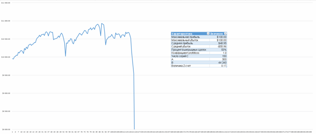
Or here’s a negative z-count:

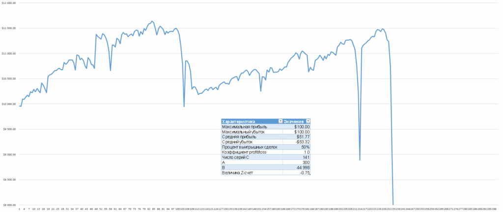
And lastly, another system with a suitable positive z-count:

Note that we use lot doubling immediately after the first losing trade. It is possible, for example, to apply the martingale mode after two or three losses in a row, which will significantly reduce drawdowns and increase the reliability of such systems. In addition, it is worth to think in more detail about the martingale system itself. For example, keep increasing the lot until the system recovers all previous losses.

Determined traders with a positive Z-score for their systems can turn this fact into cash if they are deliberate in their own money management approaches. As you and I have seen, even a losing system with a positive z-score over 2 can be made profitable. However, you should be very careful with such a dangerous method of money management as martingale. It can turn a losing system into a profitable one, as we have seen, but it can also easily turn a profitable system into a losing one. Therefore, to determine whether a system is suitable for applying martingale – it is simply necessary to use a z-count. In addition, when calculating the z-calculation it is worth taking as large a sample as possible, because the cost of error can be very high.

Finding out the z-count of a trading system is one of the best steps you can take. It will allow you to extract additional profits from the system without changing any of the parameters after a trade entry signal. It is also one of the most direct ways in which traders can turn knowledge into money.

Trading approaches of increasing the lotness in a series of profitable trades in systems with a negative Z value show very good results when combined with the technique of using moving averages of capital. The interaction of these methods allows to use the huge potential of series of profitable trades. The tactic of reducing the volume of open positions when the Z value is negative can significantly reduce the risks of your trading method.

Also, now you know what systems to look for to apply such dangerous techniques as martingale, in order to maximize (as much as possible) to protect yourself from losing your deposit. All this will give you the opportunity to increase the profitability of your trading and significantly reduce the risks, using simple mathematical calculations. At the same time, your trading system itself will not be subject to any changes. This is the most effective way to turn your theoretical knowledge about money management into real money.

In conclusion, I would like to remind you that many successful traders assure you that money management is the “holy grail” in the forex market and it is the use of rules and techniques of money management and risk control that distinguishes successful traders from the losing masses.