Laguerre Indicator - The Honor and Merit of Oscillators

Hello, fellow forex traders.

One of the most unpleasant aspects of trading when using indicator-based technical analysis is the balance between smoothing and lag. To filter out sharp noise, you have to increase the smoothing period, but then when the trend changes, the signal will lag. The less smoothing there is, the more false signals will come in. So how can you minimize the impact of noise and at the same time not miss the start of a new trend? The Laguerre indicator, which we will discuss today, will help us with this.

Platform: Metatrader 4
Currency pairs: any
Timeframe: any
Trading time: depends on your strategy
Recommended brokers: Alpari, Forex4you

The Laguerre indicator became fairly well known starting in the early 2000s, when John Ehlers described an interesting price-smoothing algorithm in his book "Cybernetic Analysis for Stocks and Futures." Ehlers is an engineer by training, and in the 1970s he worked on creating equipment designed to process aerospace signals. It was precisely this work of his that served as the basis for creating the Laguerre indicator.

Ehlers is a proponent of cycle theory, and for the development of the Laguerre indicator he used maximum entropy spectral analysis developed by geophysicists. In short, the formulas Ehlers used to calculate the indicator come down to estimating future spectra on the basis of a minimal data set. According to another theory, the appearance of the indicator is linked to the equation of the famous French mathematician Laguerre. In any case, let us better test it in action.

The Laguerre indicator is an excellent indicator for use in trend trading. Traders like it because it shows market cycles on the selected chart period better than most standard indicators from the MT4 platform set. This indicator shows the beginning and end of microtrends very well, which means it will be of interest first and foremost to swing traders and scalpers. Of course, the indicator by itself is by no means a standalone trading system, but in combination with other indicators and methods of technical analysis, Laguerre can produce a decent result.

In fact, this indicator is one of the simplest that Ehlers developed. If you visit the author's website, you can see many much more complex developments, including leading indicators with very complex calculation algorithms.

Below you can read a translation of John F. Ehlers' article "Time Warp," which explains the operating principle of the indicator in more detail. Or you can immediately move on to the section about using the Laguerre indicator in trading.

One of the most unpleasant tasks of technical analysis is avoiding trading on false signals of a trend beginning. To avoid these signals, a moving average is smoothed. But at the same time, the lag caused by smoothing often leads to a catastrophic reduction in signal effectiveness. Thus, the dilemma is this: how can we balance smoothing against acceptable lag? In this article, you will get new tools for solving the smoothing problem more effectively, and the lag problem associated with it. In particular, you will learn about the best smoothing filters and the new modified high-speed Laguerre RSI technical analysis indicator.

A moving average is a simple indicator with a period set in the settings.

It averages the data over the number of candles specified in the settings. Then it shifts forward by one bar and again shows the arithmetic mean of the new set of data (sample). Then everything repeats. In fact, with each shift only the oldest value is removed and one new one is added. In any case, the arithmetic mean is determined for a fixed period. The mean value continuously moves forward one after another. This is how the moving average "moves."

A programmer looks at this process somewhat differently. He sees that the data descend to a fixed delay line that is tapped to obtain the result of each sample, and the results of such tapping are summed to obtain the moving average. This process is shown in the diagram in Fig.1 for a moving average with a period of 4 candles. In Figure 1, the symbol Z^-1 means that there is one unit of delay. For daily charts, the shift will be one day. The characteristic of the filter from the point of view of the Z-transform is as follows:

H(z) = 1 + Z^-1 + Z^-2 + Z^-3

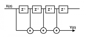
Figure 1. Moving average diagram

The moving average equation in EasyLanguage format:

Filt = (Price + Price + Price + Price) / 4;

That is, the old data from the last sample are gradually averaged in order to achieve the filtered result.

Programmers prefer the tapped delay line concept because more generalized FIR filters (finite impulse response) can be developed by changing the relative amplitudes of the samples. For example, if we wanted to give the two middle samples twice the weight compared with the freshest and the oldest values in our 4-sample example, then the diagram would look as shown in Figure 2.

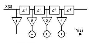
Figure 2. Diagram of a four-element finite impulse response filter (FIR filter)

The equation of the FIR filter, in EasyLanguage format, will be as follows:

Filt = (Price + 2*Price + 2*Price + Price) / 6;

The multipliers placed before the prices are called the filter coefficients. Please note that the filter is always normalized to the sum of the coefficients. This normalization is carried out in such a way that the resulting value will be the same as the original one if all samples have identical values.

The best way to compare the resulting values of the moving average and the FIR filter is to study their frequency response.

Since we are dealing with sampled data, the highest frequency we can consider is two samples per cycle. This is called the Nyquist frequency (half the sampling frequency). Thus, on daily charts, a cycle consisting of two bars operates at the Nyquist frequency, which has a normalized frequency of 1. A cycle consisting of four bars has a normalized frequency of 0.5. The general relationship between the cycle period and the normalized frequency is:

Frequency = 2 / Period

Based on this idea, the frequency response of the four-bar moving average is shown in Figure 3. The amplitude is expressed in decibels, using a logarithmic scale where 0 is the largest undamped amplitude. Since this occurs on the left side of the frequency range, we know that the gain of the filter at zero frequency is zero. Note that the 2-bar cycle and the 4-bar cycle are cut out exactly by the moving average. The filtering between the 2-bar and 4-bar cycles is reduced by only a little more than 10 dB from the zero-frequency gain.

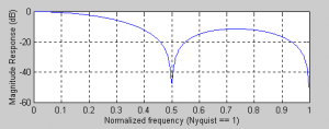
Figure 3. Frequency response of a moving average with a four-bar period

Figure 4 shows the frequency response of the FIR filter presented in Figure 2. Manipulating the coefficients improved the filtering, which becomes more than 20 dB. Nevertheless, the frequencies with the minimum value shifted to the level of a 3-bar cycle. That is, the filter's frequency range is wider than the frequency range of the moving average. A wider frequency range means that higher-frequency components can pass through the filter, and thus the FIR filter will be less smoothed than a moving average of the same length.

The FIR filter can be applied for the purpose of additional smoothing by means of a larger filter. Nevertheless, the lag in the FIR filter is approximately half the length of the filter. The result is that if we want to achieve greater smoothing, we must accept additional lag in ordinary filters.

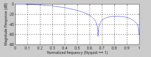
Figure 4. Frequency response of a four-element FIR filter

To describe the transfer characteristic of the filter, ordinary filters use the Z transform, where Z-1 denotes a unit delay. For arithmetic transformation there exists a semi-infinite number of orthonormal functions. One such function is formed from the Laguerre polynomial. The mathematical expression for the result of the k-th order Laguerre transfer is as follows:

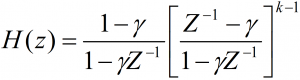
The Laguerre transform can be represented as an EMA low-pass filter (the first term), followed by a sequence of phase filter instead of unit delay (the k-1 term). All terms have exactly the same damping coefficient y. By studying the frequency response, we see that these are phase filters. If the frequency is zero, the term Z^-1 has the value 1, and therefore the term takes the value (1- y)/(1- y) = 1. Likewise, when the frequency is infinite, Z^-1 has the value -1, and therefore the term takes the value (-1- y)/(1+ y) = -1. The term has unit gain at all frequencies from zero to infinity and therefore is a phase element. Nevertheless, the phase from its original to resulting value shifts across the frequency range, because of which the delay is a variable dependent on frequency. The extent to which the delay is variable depends on the magnitude of the damping coefficient y.

For example, Figure 5 shows the lag or group delay for y = 0.6  and g = 0.8.

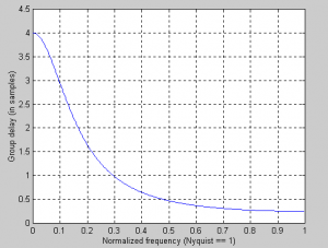
y = 0.6

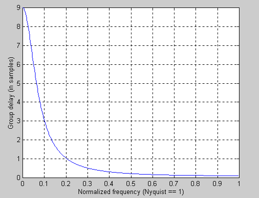
y = 0.8

Figure 5. The delay of the phase filter is a function of frequency and the damping coefficient

Thus, we can make a filter using Laguerre elements instead of a unit delay, whose coefficients are the same /6 as those of the FIR filter.

The only difference is that we distorted the time between the periods of the delay line. The Laguerre filter diagram is shown in Figure 6.

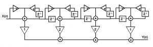
Figure 6. Laguerre filter diagram

Figure 7 shows EasyLanguage code for a four-element Laguerre filter. L0 is the resulting value of the first element, as well as an ordinary EMA. The next three elements are identical in their form. The four elements of the Laguerre delay line are summed in exactly the same way as if it were possible to sum a linear delay line for an FIR filter. The resulting Laguerre value is the "Filt" variable. For comparison, an FIR filter of the same length is also calculated.

Inputs: Price((H+L)/2),

gamma(.8);

Vars:   L0(0),

L1(0),

L2(0),

L3(0),

Filt(0)

FIR(0);

L0 = (1 - gamma)*Price + gamma*L0;

L1 = -gamma*L0 + L0 + gamma*L1;

L2 = -gamma*L1 + L1 + gamma*L2;

L3 = -gamma*L2 + L2 + gamma*L3;

Filt = (L0 + 2*L1 + 2*L2 + L3) / 6;

FIR = (Price + 2*Price + 2*Price + Price) / 6;

Plot1(Filt, "Filt");

Plot2(FIR, "FIR");

Figure 7. EasyLanguage code for the Laguerre filter

Figure 8 shows the results of the Laguerre filter and the FIR filter.  Remember: both filters have the same lengths. The FIR filter (green line) has a lag of only 1.5 bars and only moderately smooths the price data. On the other hand, the Laguerre filter (red line) is significantly smoother and also has a more pronounced lag. You can reduce the smoothing and lag by decreasing the damping factor. When the damping factor is reduced to zero, the Laguerre filter becomes identical to the FIR filter. This is a simple way to control the moving average. And it still uses only a few data samples for the calculation.

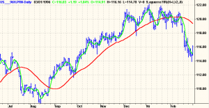
Figure 8. The four-element Laguerre filter is much smoother than the regular four-element FIR filter

The story does not end with ordinary filters. As I like to say: "Truth and science always triumph over ignorance and superstition." If we can create superior smoothing using very short filters, then we should also be able to create superior indicators using very short-term data. Using short-term data means that we can make indicators more sensitive to price changes. The Laguerre RSI indicator will be used as an example.

Welles Wilder defined the RSI indicator as:

RSI = 100 - 100 / (1 + RS)

where RS = (Closes Up) / (Closes Down) = CU/CD

RS is an abbreviation for Relative Strength. CU represents the sum of closing price differences over the observation period when that difference is positive. CD represents the sum of closing price differences over the observation period when that difference is negative, but the sum is expressed as a positive number. Substituting CU/CD into the formula and simplifying the RSI equation, we get

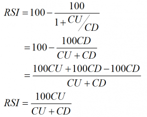
In other words, RSI is the percentage of the sum of closing price deltas with a positive difference relative to the sum of all closing price deltas over the observation period.

In the EasyLanguage code (see Figure 9), I generated the RSI indicator using Laguerre time rather than linear time, using only four data samples. In this case, I used a damping factor of 0.5, but you can adjust your damping time so that it best suits your own trading.

Inputs: gamma(.5);

Vars:   L0(0),

L1(0),

L2(0),

L3(0),

CU(0),

CD(0),

RSI(0);

L0 = (1 – gamma)*Close + gamma*L0;

L1 = - gamma *L0 + L0 + gamma *L1;

L2 = - gamma *L1 + L1 + gamma *L2;

L3 = - gamma *L2 + L2 + gamma *L3;

CU = 0;

CD = 0;

If L0 >= L1 then CU = L0 - L1 Else CD = L1 - L0;

If L1 >= L2 then CU = CU + L1 - L2 Else CD = CD + L2 - L1;

If L2 >= L3 then CU = CU + L2 - L3 Else CD = CD + L3 - L2;

If CU + CD <> 0 then RSI = CU / (CU + CD);

Plot1(RSI, "RSI");

Plot2(.8);

Plot3(.2);

Figure 9. EasyLanguage code for the Laguerre RSI indicator

Figure 10 shows an example of the response of the four-element Laguerre RSI indicator, located below the price chart. Signal levels of 20% and 80% are also plotted on the indicator. Note that the RSI, as a rule, moves from one extreme value to another and that recovery occurs quickly, at each price reversal.

The Laguerre RSI indicator is usually used to buy after the line crosses the 20% level from below upward, and to sell after the price crosses the 80% level from above downward. But, as with the regular RSI, it is also possible to create more complex trading rules.

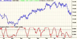
Figure 10. The Laguerre RSI indicator reacts quickly to price changes

Applying more complex rules is not necessary at all, since the Laguerre RSI system turned out to be the most useful among all the systems registered at www.wellinvested.com, its annual return, according to estimates by AKSYS Ltd., amounted to 118.3%. The WellInvested.com site presents a wide selection of systems for automated trading that are applied to most exchange-listed stocks and futures. The search engine on the site may prove very interesting. For example, for a given symbol you can find the highest-performing systems, and for a given system you can find the highest-performing symbols. It turns out that two Laguerre systems were the most productive in the famous contract with Diamond Trust in 2002 (see Figure 11).

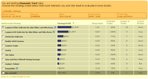
Figure 11. A screenshot taken from www.wellinvested.com demonstrates the Laguerre trading systems that were the most productive in the contract with Diamond Trust in 2002

The Laguerre transformation introduces a peculiar time distortion into calculations. As a result, the delay of the low-frequency components of price is significantly higher than that of its high-frequency components. Thanks to this feature, it is possible to create smoothing filters that require only a small amount of input data to operate.

In a similar way, through time distortion it is possible to develop indicators even with only a small sample at one's disposal. Since these indicators are created on the basis of a small sample, they will be more sensitive to newer prices.

Greater sensitivity helps reduce the response time for opening a position, and reduced lag, accordingly, has a positive effect on the profitability of your trading.

John F. Ehlers

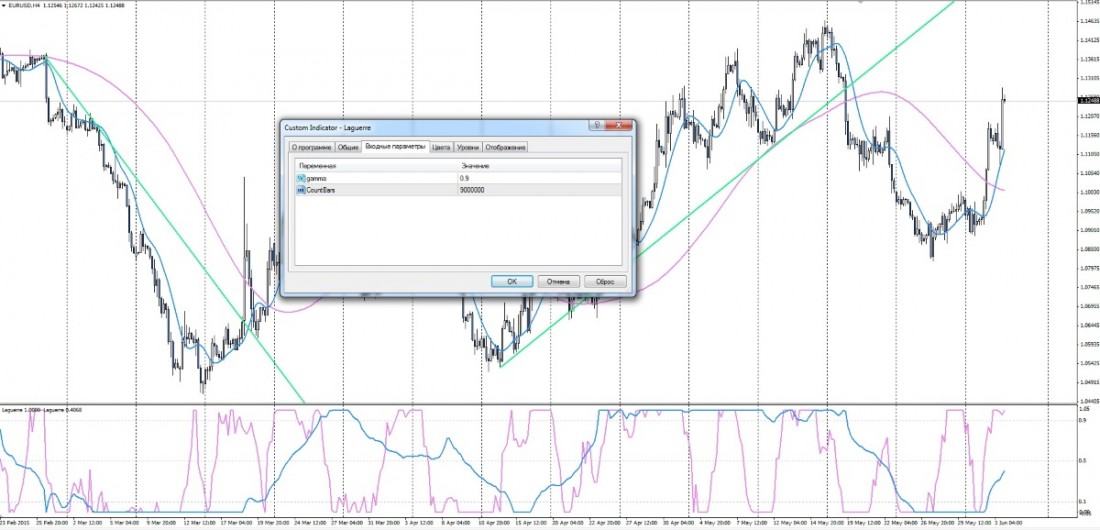
gamma (default = 0.7) is the coefficient for calculating the indicator levels. The higher the gamma , the smoother the output line will be.

CountBars (default = 950) is the maximum number of chart bars on which the indicator will be calculated.

Despite the fact that the Laguerre indicator is considered a trend indicator, it is built on the oscillator principle, where the final values are within certain limits. In our case, this is the interval from 0 to 1.

The simplest option for using it is buying when the line crosses 0.2 from bottom to top and selling when the line crosses 0.8 from top to bottom. You can also use the 0.5 smoothed indicator line to filter trades by the system: if Laguerre is below 0.5, we consider only sells, if above, only buys. Or consider the possibility of exiting buys if the Laguerre indicator crossed the 0.5 or 0.8 line from top to bottom and the possibility of exiting sells when the 0.2 or 0.5 line is crossed from bottom to top.

Let us look at a simple example of the practical use of the Laguerre indicator in a strategy for trading on the Forex currency market. John Ehlers himself noted that cycles in financial markets must be applied in combination with trend methods, so for the example I will take two moving averages. You can experiment with trend lines, channels, and other trend indicators as well.

Let us take two moving averages and enter when they cross, filtering the entry with two Laguerre indicators: one with gamma = 0.6, and the second 0.8. If the fast moving average crosses the slow one upward, the fast Laguerre is above the 0.8 level, and the slow one started to rise from below and crossed the 0.2 level, we enter buys. Exiting buys can be done when the slow Laguerre indicator crosses the 0.8 level from top to bottom. For sells, everything is the opposite. Such a strategy, together with a trailing stop, can work quite normally on the H4 period.

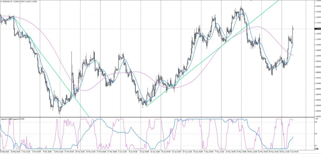
I repeat, the Laguerre indicator is not a full-fledged trading system, so it should be used together with other indicators or methods of technical analysis. Nevertheless, on higher periods (from D1 and above), you can even manage with two Laguerre indicators - a fast and a slow one. The slower one becomes the trend direction indicator, while the faster one generates signals for entering the market.

In addition, interesting results are obtained when working with trend lines and Laguerre indicator divergences. Usually, the indicator forms a divergence with the price shortly before the breakout of the existing trend line and a trend break.

The Laguerre indicator is a trend indicator that displays a trend line in a separate window. It can be used as a confirming signal for entering the market, as well as a separate trading system. This indicator is very easy to use. It can be used equally successfully both for exiting a trade and as a signal for entry.

At the same time, the author still could not completely eliminate the main problem of all indicators - the lag problem. And nevertheless, the Laguerre indicator gives signals more often and more accurately than most standard oscillators, while the number of false signals is noticeably lower than that of the same stochastic.

Discussion on the forum

Expert Advisor based on the indicator

Respectfully, Dmitry aka Silentspec
TradeLikeaPro.ru